写在前头
译者水平有限, 有些地方读起来难免会感到怪怪的, 还请各位见谅。如果您遇到什么看不懂的地方或者乱七八糟的句子, 那么您很可能是辣鸡翻译的受害者, 这时候请不要犹豫, 直接去阅读原文 自救。如果您愿意帮助我改进这个翻译, 请直接在页面底部留言 或发送邮件 到zgxmy@126.com , 万分感激!!!
目录:1. Overview 概述 2. Motion Blur 动态模糊 3. Bounding Volume Hierarchies 层次包围盒 4. Solid Texture 固体贴图 5. Perlin Noise 柏林噪声 6. Image Texture Mapping 图像纹理映射 7. Rectangles and Lights 矩形和光源 8. instance 实例 9. volumes 体积体 10. A Scene Testing All New Features 一个测试所有新特性的场景 译者后记
1. 概述 在Ray Tracing in One Weekend 中, 你实现了一个暴力的光线路径追踪器。在本部分中, 我们将加入纹理, 体积体(例如烟雾), 矩形, 实例, 光源, 并用BVH来包裹我们的物体。当你完成这些后, 你将拥有一个“真正的”光线追踪器。
在光线追踪方面, 具有启发性的一点是, 许多人(包括作者本人)相信大多数用来优化的代码只会让程序更复杂, 而并不会提升太多的运行速度。我在这本迷你书中将采取最简单直接的方式来实现代码。如果你想看复杂的优化版本, 请点击这里 。并且我在这里建议读者不要自己过早的去优化。如果说程序在执行时间上来看并没有太大的变化, 那么它就并不需要你去优化。直到最后所有的功能都被实现前, 你可以一直就这样往里面添加代码。
本书中最难的两部分是BVH和柏林噪声贴图。所以我将标题取名为“一周”而不是像上一本一样的“一个周末”。如果你想一个周末搞定这本书, 那么你可以把这两个部分留到最后。这本书中提到的概念, 各章节的顺序并不是很重要, 没有BVH和柏林噪声贴图你仍然能渲染出属于自己漂亮的Cornell Box!
1.1 致谢 感谢 Becker 对草稿的许多建设性意见。感谢 Matthew Heimlich 指出一个严重的动态模糊的错误。感谢 Andrew Kensler, Thiago Ize, and Ingo Wald 对ray-AABB 测试的建议。 感谢 David Hart and Grue Debry 对细节补完上的帮助。 感谢 Jean Buckley 的编辑, 感谢 Dan Drummond 修复代码bug, 感谢 Steve Hollasch and Trevor David Black 将本书翻译为 Markdeep 并挪到该网页 上。
2. 动态模糊 当你在做光线追踪时, 想要更好的出图质量就意味着更多的程序运行时间。例如上一本书中的反射部分和镜头散焦模糊中, 你需要对每个像素进行多重采样。当你决定在这条路上走得更深一些时, 好消息来了: 几乎所有的特效都能这样暴力实现。动态模糊也是属于能这样实现的特效之一。想象一个真实世界的摄像机, 在快门打开的时间间隔中, 摄像机和物体都有可能移动。那拍出来的结果肯定是这个运动过程每一帧的平均值, 或者说, 一团糊了。我们可以用随机的方法在不同时间发射多条射线来模拟快门的打开。只要物体在那个时间处于其正确的位置, 那么我们就能得出这条光线在那个时间点的精确平均值。这就是为什么随机光追看上去很简单的原因。
一个基础的思路是, 在快门打开时, 随着时间变化随机生成光线, 并同时发出射线与模型相交。一般来说我们让摄像机和物体同时运动, 并让每一条射线都拥有自己存在的一个时间点。这样光线追踪器的“引擎”就能确定, 对于指定的某条光线来说, 在该时刻, 物体到底在哪儿。求射线与球相交的部分写法和之前并没有太多区别。
为了实现刚刚的思路, 我们首先要让每条光线都能储存自己所在的时刻, 就像这样:
ray.h diff 1 2 3 4 5 6 7 8 9 10 11 12 13 14 15 16 17 18 19 20 class ray {public :ray () {}ray (const vec3& origin, const vec3& direction, double time = 0.0 )orig (origin), dir (direction), tm (time)vec3 origin () const { return orig; }vec3 direction () const { return dir; }double time () const return tm; }vec3 at (double t) const {return orig + t*dir;public :double tm;
现在我们需要让摄像机在time1到time2的时间段中随机生成射线。光线的生成时刻是让camera类自己来运算追踪呢, 还是说可以让用户来自行指定光线在哪个时刻生成比较好呢? 当出现这样的疑问时, 我喜欢让构造函数更加复杂,同时调用起来会更加简单。所以我让camera类来储存着两个变量。但这只是我的个人喜好。camera类并不需要太多修改, 因为现在它不会动, 只会在一个时间段内发出射线。
camera.h diff 1 2 3 4 5 6 7 8 9 10 11 12 13 14 15 16 17 18 19 20 21 22 23 24 25 26 27 28 29 30 31 32 33 34 35 36 37 38 39 40 41 42 43 44 45 46 47 class camera {public :camera (double vfov, double aspect, double aperture, double focus_dist, double t0 = 0 , double t1 = 0 2 ;auto theta = degrees_to_radians (vfov);auto half_height = tan (theta/2 );auto half_width = aspect * half_height;unit_vector (lookfrom - lookat);unit_vector (cross (vup, w));cross (w, u);2 *half_width*focus_dist*u;2 *half_height*focus_dist*v;ray get_ray (double s, double t) {random_in_unit_disk ();x () + v * rd.y ();return ray (random_double (time0, time1)public :double lens_radius;double time0, time1;
我们还需要一个运动中的物体。我建立了一个新的sphere类, 让它的球心在time0到time1的时间段内从center0线性运动到center1。超出这个时间段, 这个球心依然在动, 【译注:就是说在做线性插值的时候t可以大于1.0 也可以小于0】 , 所以这里的两个时间变量和摄像机快门的开关时刻并不需要一一对应。
move_sphere.h method 1 1 2 3 4 5 6 7 8 9 10 11 12 13 14 15 16 17 18 19 20 21 22 class moving_sphere :public hittable {public :moving_sphere () {}moving_sphere (double t0, double t1, double r, shared_ptr<material> m)center0 (cen0), center1 (cen1), time0 (t0), time1 (t1), radius (r), mat_ptr (m)virtual bool hit (const ray& r, double tmin, double tmax, hit_record& rec) const vec3 center (double time) const ;public :double time0, time1;double radius;vec3 moving_sphere::center (double time) const {return center0 + ((time - time0) / (time1 - time0))*(center1 - center0);
另外一种让球随着时间动起来的方法是, 取代先前新建一个动态球类的做法, 只留一个球类, 让所有的球都动起来, 只是那些静止的球起点与终点位置相同。我在第一种方案和第二种方案间反复很跳。所以就请你们自己根据自己的喜好来选择吧。球与光线求交的代码几乎没有改变: 只要把center改成一个插值函数center(time)就行了
sphere.h method 2 diff 1 2 3 4 5 6 7 8 9 10 11 12 13 14 15 16 17 18 19 20 21 22 23 24 25 26 27 28 29 30 31 32 33 34 bool moving_sphere::hit ( const ray& r, double t_min, double t_max, hit_record& rec) const origin () - center (r.time ());auto a = r.direction ().length_squared ();auto half_b = dot (oc, r.direction ());auto c = oc.length_squared () - radius*radius;auto discriminant = half_b*half_b - a*c;if (discriminant > 0 ) {auto root = sqrt (discriminant);auto temp = (-half_b - root)/a;if (temp < t_max && temp > t_min) {at (rec.t);center (r.time ())) / radius;set_face_normal (r, outward_normal);return true ;if (temp < t_max && temp > t_min) {at (rec.t);center (r.time ())) / radius;set_face_normal (r, outward_normal);return true ;return false ;
请确保你的材质在运算光线散射时, 散射光线与入射光线所存在的时间点相同。
material.h diff 1 2 3 4 5 6 7 8 9 10 11 12 13 14 15 class lambertian :public material {public :lambertian (const vec3& a) : albedo (a) {}virtual bool scatter ( const ray& r_in, const hit_record& rec, vec3& attenuation, ray& scattered ) const random_unit_vector ();ray (rec.p, scatter_direction, r_in.time ());return true ;
下面的代码是在上本书结尾处最终场景的例子上加以改动, 使其中漫反射材质的球动起来。(想象一下摄像机的快门在time0时打开, 在time1时关闭)每个球的中心在time0到time1的时间段内从原始位置$\mathbf{C}$线性运动到$\mathbf{C} + (0, r/2, 0)$, 其中r是[0,1)之间的随机数。
main.cc 1 2 3 4 5 6 7 8 9 10 11 12 13 14 15 16 17 18 19 20 21 22 23 24 25 26 27 28 29 30 31 32 33 34 35 36 37 38 39 40 hittable_list random_scene () {add (make_shared<sphere>(vec3 (0 ,-1000 ,0 ), 1000 , make_shared<lambertian>(vec3 (0.5 , 0.5 , 0.5 ))));int i = 1 ;for (int a = -10 ; a < 10 ; a++) {for (int b = -10 ; b < 10 ; b++) {auto choose_mat = random_double ();vec3 center (a + 0.9 *random_double(), 0.2 , b + 0.9 *random_double()) ;if ((center - vec3 (4 , .2 , 0 )).length () > 0.9 ) {if (choose_mat < 0.8 ) {auto albedo = vec3::random () * vec3::random ();add (make_shared<moving_sphere>(vec3 (0 , random_double (0 ,.5 ), 0 ), 0.0 , 1.0 , 0.2 ,else if (choose_mat < 0.95 ) {auto albedo = vec3::random (.5 , 1 );auto fuzz = random_double (0 , .5 );add (0.2 , make_shared<metal>(albedo, fuzz)));else {add (make_shared<sphere>(center, 0.2 , make_shared<dielectric>(1.5 )));add (make_shared<sphere>(vec3 (0 , 1 , 0 ), 1.0 , make_shared<dielectric>(1.5 )));add (make_shared<sphere>(vec3 (-4 , 1 , 0 ), 1.0 , make_shared<lambertian>(vec3 (0.4 , 0.2 , 0.1 ))));add (make_shared<sphere>(vec3 (4 , 1 , 0 ), 1.0 , make_shared<metal>(vec3 (0.7 , 0.6 , 0.5 ), 0.0 )));return world;
并使用以下的摄像机参数:
main.cc 1 2 3 4 5 6 7 8 9 const auto aspect_ratio = double vec3 lookfrom (13 ,2 ,3 ) ;vec3 lookat (0 ,0 ,0 ) ;vec3 vup (0 ,1 ,0 ) ;auto dist_to_focus = 10.0 ;auto aperture = 0.0 ;camera cam (lookfrom, lookat, vup, 20 , aspect_ratio, aperture, dist_to_focus, 0.0 , 1.0 ) ;
你将会得到类似下面的结果:
3. 层次包围盒 这部分是书中最难,也是与我们正在写的光线追踪器关联最深的一部分。我把这部分放在这么前面, 是因为它改写了hittable的部分代码, 程序运行起来更加的快了。而且当我们后面添加三角形和箱子类的时候, 我们也不必回来改写hittable了。
光线的求交运算一直是光线追踪器的主要时间瓶颈, 并且运行时间与场景中的物体数量线性相关。使用遍历反复查找同一个模型会有许多多余的计算, 所以我们应该用二叉搜索的方法来加速查找。我们对每个模型都射出了成千上万的射线, 我们可以对模型的排序进行模拟, 每一次光线求交都是一个亚线性(subliner)的查找 【译注:亚线性指参数的指数小于1, 即不到线性, 平衡查找树的时间复杂度为O(log2(n))】 。最常见的两种排序方法是 1) 按空间分割 【译注: 如KD树、八叉树】 2) 按物体分割。后者一般来说实现起来更简单并且对大多数模型来说运行速度都不错。
包围盒的核心思想是去找到一个能包围所有物体的盒子。举例来说, 假设你计算了一个包围10个物体的大球, 那么任何射不到这个大球的射线, 它都射不到球里面的那10个物体。反之亦然, 如果射线碰到大球了, 那么它和里面那10个物体都有可能发生关系。所以包围盒的代码看上去总是这样的:
1 2 3 4 if (ray hits bounding object)return whether ray hits bounded objectselse return false
记住, 我们的核心思想是把很多很多物体分割为子集。我们并不划分屏幕或者是空间。每个物体都只在一个包围盒里面, 并且这些包围盒还可以重叠。
为了做到每次光线求交都是一个亚线性的查找, 我们需要用包围盒构建出层级(hierarchical)。举个例子, 如果我们把一堆物体分成两队, 红队和蓝队, 并使用方方正正的包围盒来包围他们, 你将看到如下场景:
注意蓝盒子和红盒子现在都在紫盒子里面, 他们可以重合, 并且无序 —— 他们都平平等等的躺在紫盒子的肚子里。所以图片里右边的那颗树并没有什么左子树右子树的概念 【译注: 作者这里只是想强调他们属于同一层, 地位平等。等待会实际写这个二叉查找树的时候还是会有左子树右子树的】 , 这两个分支是同级的。代码看起来是这样的:
1 2 3 4 5 6 if (hits purple)if (hit0 or hit1)return true and info of closer hitreturn false
为了能使上述代码良好的跑起来, 我们需要好好规划一下怎么分堆。还得想想怎么去检测光线和包围盒相交。求交计算一定要高效, 并且包围盒要尽量密集。很对大多数模型来说, 轴对齐的包围盒比其他种类的包围盒效果更好。但是当你遇到更复杂的模型种类时, 你就先别想着用这种方法了。
从现在开始, 我们会把轴对齐的包围盒叫成矩形平行管道(讲真的, 这才是他本来该有的精确描述), 或者还是叫他 AABB 吧 。你想用啥方法去算光线和AABB是否相交都行。我们现在只要能判断我们能不能射中这个AABB就行了。和击中那些会在屏幕上显示出来的物体时不同, 射线与AABB求交并不需要去获取那些法向啊交点啊这些东西, AABB不需要在屏幕上渲染出来。
大多数人采用一个叫堆叠法(slab)的方法。显然一个n维的AABB盒是由n个平行线所截的区间的重叠拼出来的区域 【译注: 这里看图就行了, 别看字】 , 我们管这个叫”slab”。一个区间就是两个端点间的距离。比如对于$x$, $3<x<5$, 或者更加简洁的 $x$ 属于 $(3,5)$ 。在二维的情况下, 两段区间重叠的部分就是一个二维的AABB(一个矩形):
对于检测射线是否射入一段区间来说, 我们首先要看看射线有没有射入这个区间的边界。还是拿二维来举例子, 这是光线变量t0, t1。(在光线和目标平面平行的情况下, 因为并没有交点, 这两个变量将未定义)
在三维的情况下, 这些射入的边界不再是一条线, 而是一个平面。 这两个边界平面的方程分别是 $x=x_0$ 和 $x=x_1$。那么怎样来计算射线和平面相交呢? 让我们回想一下上一本书中我们给出的, 点p关于参数t的方程
$p(t) = A + t·B$
这个等式用在三个坐标轴上都行, 比如
$x(t) = A_x + t·B_x$
然后我们把这个方程和平面方程$x=x_0$联立, 使得存在一个值t, 满足下面方程:
$x_0 = A_x + t_0·B_x$
我们稍稍变下形:
$t_0=\frac{x_0-A_x}{B_x}$
同理, 对于$x_1$的那个平面来说:
$t_1=\frac{x_1-A_x}{B_x}$
把这个1D的等式运用到我们AABB求交运算的关键是, 你需要把n个维度的t区间重叠在一起。举例来说, 在2D情况下, 绿色的t区间和蓝色的t区间发生重叠的情况如下:
【译注: 这张图挺好的, 上面的那条射线, 蓝色与绿色部分没有重叠, 很自然的就没有穿过这个AABB矩形, 下面那条射线发生了重叠, 说明射线同时传过了蓝色区域和绿色区域, 即穿过了AABB矩形。注意对每一个维度来说, 这里我们解出来的t0, t1都表示直线上一个固定的点的位置, 所以我们可以自然地按照维度拆分计算, 然后在通过t这个统一的标识进行求交运算】
用代码表示”区间们是否重叠”看上去会是这样:
1 2 3 compute (tx0,tx1)compute (ty0,ty1)return overlap?( (tx0, tx1), (ty0, ty1))
这看上去真是简洁! 而且放到3D的情况下依旧适用, 所以大家都爱堆叠法:
1 2 3 4 compute (tx0, tx1)compute (ty0, ty1)compute (tz0, tz1)return overlap?( (tx0, tx1), (ty0, ty1), (tz0, tz1))
当然我们还要对它做一些限制, 这会使它看上去没有一开始那么简洁。首先, 假设射线从$x$轴负方向射入, 这样前面compute的这个区间$(t_x0,t_x1)$就会反过来了, e.g. $(7, 3)$。第二, 除数为零时我们会得到无穷, 如果射线的原点就在这个堆叠的边界上, 我们就会得到$NaN$。不同的光线追踪器的AABB部分解决上述问题的方法多种多样。(这里还有一些矢量平行加速的方面比如SIMD, 我们本书中不讨论。如果你想走得更远些, 使用这种方法加速的话, Ingo Wald的论文 将是个不错的选择)。对我们来说, 这并不是一个运算的主要瓶颈。所以直接让我们用最快捷最简单的方式搞起来吧! 首先我们来看看需要计算的这些区间。
$t_x0 = \frac{x_0-A_x}{B_x}$
我们的麻烦是一些射线恰好$B_x = 0$, 这样就会有除数为0的错误。一些光线在堆叠的里面, 一些不在。浮点$0$在 IEEE 工程标准下是有正负号的。好消息是, 在$x_0$到$x_1$区间内, $t_x0$与$t_x1$要么同为$\infty$要么同为$-\infty$。所以使用 min 与 max 函数就能得到正确的结果:
$t_x0 = min(\frac{x_0-A_x}{B_x},\frac{x_1-A_x}{B_x})$
现在只剩下分母$B_x = 0$并且$x_0 - A_x = 0$和$x_1 - A_x = 0$这两个分子之一为零的特殊情况了。这样我们会得到一个NaN【译注: 0/0 = NaN】 。这种情况我们认为他射中了或者没射中这个区域都行。我们过会儿再来解决这个问题。
现在让我们先来看看overlap函数, 假设我们能保证区间没有被倒过来(即第一个值比第二个值小), 在这种情况下我们 return true, 那么一个计算$(d,D)$和$(e,E)$的重叠区间$(f,F)$的函数看上去是这样的:
1 2 3 4 bool overlap (d, D, e, E, f, F) f = max (d, e)min (D, E)return
如果这里出现了任何的NaN, 比较结果都会 return false, 所有如果考虑到那些擦边的情况, 我们要保证我们的包围盒有一些内间距(而且我们也许理应这么做, 因为在光线追踪中所有的情况最终都会发生)。把三个维度都写在一个循环中并传入时间间隔$t_min$,$t_max$我们得到:
aabb.h 1 2 3 4 5 6 7 8 9 10 11 12 13 14 15 16 17 18 19 20 21 22 23 24 25 26 27 #include "rtweekend.h" class aabb {public :aabb () {}aabb (const vec3& a, const vec3& b) { _min = a; _max = b;}vec3 min () const {return _min; }vec3 max () const {return _max; }bool hit (const ray& r, double tmin, double tmax) const for (int a = 0 ; a < 3 ; a++) {auto t0 = ffmin ((_min[a] - r.origin ()[a]) / r.direction ()[a],origin ()[a]) / r.direction ()[a]);auto t1 = ffmax ((_min[a] - r.origin ()[a]) / r.direction ()[a],origin ()[a]) / r.direction ()[a]);ffmax (t0, tmin);ffmin (t1, tmax);if (tmax <= tmin)return false ;return true ;
注意我们把cmath内置的fmax()函数换成了我们自己的ffmax()(在rtweekend中定义)。这样会更快一点, 因为我们自己写的函数并不需要考虑到NaN和其他的异常情况。来自皮克斯的Andrew Kensler在阅读我的这个求交方法时做了一些试验, 并提出了一个自己的版本。这个版本在大多数编译器上都运行的非常好。所以我采用了这个方法作为我们接下来要使用的方法。
Andrew Kensler's hit method 1 2 3 4 5 6 7 8 9 10 11 12 13 14 15 inline bool aabb::hit (const ray& r, double tmin, double tmax) const for (int a = 0 ; a < 3 ; a++) {auto invD = 1.0f / r.direction ()[a];auto t0 = (min ()[a] - r.origin ()[a]) * invD;auto t1 = (max ()[a] - r.origin ()[a]) * invD;if (invD < 0.0f )swap (t0, t1);if (tmax <= tmin)return false ;return true ;
现在我们需要加入一个函数来计算这些包裹着hittable类的包围盒。然后我们将做一个层次树。在这个层次树中, 所有的图元, 比如球体, 都会在树的最底端(叶子节点)。这个函数返回值是一个 bool 因为不是所有的图元都有包围盒的(e.g 无限延伸的平面)。另外, 物体会动, 所以他还要接收time1和time2, 包围盒会把在这个时间区间内运动的物体完整的包起来。
hittable.h diff 1 2 3 4 5 6 class hittable {public :virtual bool hit ( const ray& r, double t_min, double t_max, hit_record& rec) const 0 ;virtual bool bounding_box (double t0, double t1, aabb& output_box) const 0 ;
对一个sphere类来说, 求包围盒真的太简单了:
1 2 3 4 5 6 bool sphere::bounding_box (double t0, double t1, aabb& output_box) const aabb (vec3 (radius, radius, radius),vec3 (radius, radius, radius));return true ;
对于moving_sphere, 我们先求球体在$t_0$时刻的包围盒, 再求球体在$t_1$时刻的包围盒, 然后再计算这两个盒子的包围盒:
1 2 3 4 5 6 7 8 9 10 bool moving_sphere::bounding_box (double t0, double t1, aabb& output_box) const aabb box0 ( center(t0) - vec3(radius, radius, radius), center(t0) + vec3(radius, radius, radius)) aabb box1 ( center(t1) - vec3(radius, radius, radius), center(t1) + vec3(radius, radius, radius)) surrounding_box (box0, box1);return true ;
对于hittable_list来说, 我们可以在构造函数中就进行包围盒的运算, 或者在程序运行时计算。我喜欢在运行时计算, 因为这些包围盒的计算一般只有在BVH构造时才会被调用。
1 2 3 4 5 6 7 8 9 10 11 12 13 14 bool hittable_list::bounding_box (double t0, double t1, aabb& output_box) const if (objects.empty ()) return false ;bool first_box = true ;for (const auto & object : objects) {if (!object->bounding_box (t0, t1, temp_box)) return false ;surrounding_box (output_box, temp_box);false ;return true ;
我们需要一个surrounding_box函数来计算包围盒的包围盒。
1 2 3 4 5 6 7 8 9 aabb surrounding_box (aabb box0, aabb box1) {vec3 small (ffmin(box0.min().x(), box1.min().x()), ffmin(box0.min().y(), box1.min().y()), ffmin(box0.min().z(), box1.min().z())) vec3 big (ffmax(box0.max().x(), box1.max().x()), ffmax(box0.max().y(), box1.max().y()), ffmax(box0.max().z(), box1.max().z())) return aabb (small,big);
BVH也应该是hittable的一员, 就像hittable_list类那样。BVH虽然是个容器, 但也能对于问题“这条光线射中你了么?”做出回答。一个设计上的问题是, 我们是为树和树的节点设计两个不同的类呢, 还是用一个类加上指针来搞定。我是一个类搞定派, 所以这个类会是这样:
bvh.h 1 2 3 4 5 6 7 8 9 10 11 12 13 14 15 16 17 18 19 20 21 22 23 24 25 class bvh_node :public hittable {public :bvh_node ();bvh_node (hittable_list& list, double time0, double time1)bvh_node (list.objects, 0 , list.objects.size (), time0, time1)bvh_node (size_t start, size_t end, double time0, double time1);virtual bool hit (const ray& r, double tmin, double tmax, hit_record& rec) const virtual bool bounding_box (double t0, double t1, aabb& output_box) const public :bool bvh_node::bounding_box (double t0, double t1, aabb& output_box) const return true ;
注意我们的子节点指针是hittable*, 所以这个指针可以指向所有的hittable类。例如节点bvh_node, 或者是sphere, 或者是其他各种各样的图元。
hit 函数也是十分的直接明了: 检查这个节点的box是否被击中, 如果是的话, 那就对这个节点的子节点进行判断。【译注: 对于二叉树来说, 这样的递归结构相信大家并不陌生】
bvh.h 1 2 3 4 5 6 7 8 9 bool bvh_node::hit (const ray& r, double t_min, double t_max, hit_record& rec) const if (!box.hit (r, t_min, t_max))return false ;bool hit_left = left->hit (r, t_min, t_max, rec);bool hit_right = right->hit (r, t_min, hit_left ? rec.t : t_max, rec);return hit_left || hit_right;
任何高效的数据结构, 例如BVH, 最复杂的部分就是如何去构建他。我们会在构造函数里完成。 对于BVH来说, 很酷的一点是当你不断地把bvh_node中的物体分割成两个子集的同时, hit函数也会跟着执行。如果说你分割的算法很好, 两个孩子的包围盒都比其父节点的包围盒要小, 那么自然hit函数也会运行的很好。但是这样只是快, 并不正确, 我将在正确和快直接做取舍, 在每次分割时我沿着一个轴把物体列表分成两半。我将采用最简单直接的分割原则:
1.随机选取一个轴来分割sort()对图元进行排序
物体分割过程递归执行, 当数组传入时只剩下两个元素时, 我在两个子树节点各放一个, 并结束递归。为了使遍历算法平滑, 并且不去检查空指针, 当只有一个元素时, 我将其重复的放在每一个子树里。想象一下有三个元素, 然后仔细的一步步递归一遍有助你理解算法, 但我这里先提一下, 之后我们会优化整个算法。现在代码是这样的:
1 2 3 4 5 6 7 8 9 10 11 12 13 14 15 16 17 18 19 20 21 22 23 24 25 26 27 28 29 30 31 32 33 34 35 36 37 38 39 40 41 #include <algorithm> bvh_node (size_t start, size_t end, double time0, double time1int axis = random_int (0 ,2 );auto comparator = (axis == 0 ) ? box_x_compare1 ) ? box_y_comparesize_t object_span = end - start;if (object_span == 1 ) {else if (object_span == 2 ) {if (comparator (objects[start], objects[start+1 ])) {1 ];else {1 ];else {sort (objects.begin () + start, objects.begin () + end, comparator);auto mid = start + object_span/2 ;if ( !left->bounding_box (time0, time1, box_left)bounding_box (time0, time1, box_right)"No bounding box in bvh_node constructor.\n" ;surrounding_box (box_left, box_right);
这边做了一个物体是否有包围盒的检查, 是为了防止你把一些如无限延伸的平面这样没有包围盒的东西传进去当参数。我们现在并没有这样的图元, 所以在你手动添加这样的图元之前, 这个std::cerr并不会被执行。
现在我们需要实现std::sort()使用的比较函数。我们先判断是哪个轴, 然后对应的为我们的比较器赋值。
bvh.h 1 2 3 4 5 6 7 8 9 10 11 12 13 14 15 16 17 18 19 20 21 22 inline bool box_compare (const shared_ptr<hittable> a, const shared_ptr<hittable> b, int axis) if (!a->bounding_box (0 ,0 , box_a) || !b->bounding_box (0 ,0 , box_b))"No bounding box in bvh_node constructor.\n" ;return box_a.min ().e[axis] < box_b.min ().e[axis];bool box_x_compare (const shared_ptr<hittable> a, const shared_ptr<hittable> b) return box_compare (a, b, 0 );bool box_y_compare (const shared_ptr<hittable> a, const shared_ptr<hittable> b) return box_compare (a, b, 1 );bool box_z_compare (const shared_ptr<hittable> a, const shared_ptr<hittable> b) return box_compare (a, b, 2 );
【译注: 使用方法:在random_scene()函数最后return static_cast(make_shared(world,0,1));】
4. 纹理 在图形学中, 纹理贴图常常意味着一个将颜色赋予物题表面的一个过程。这个过程可以是纹理生成代码, 或者是一张图片, 或者是两者的结合。我们首先来使用颜色作为贴图。大多数程序员把静态rgb颜色和贴图写成两个不同的类, 以此来区分两者, 但我更加喜欢下面的做法, 因为这样就可以把任何颜色弄成一张贴图, 十分的great。
1 2 3 4 5 6 7 8 9 10 11 12 13 14 15 16 17 18 19 #include "rtweekend.h" class texture {public :virtual vec3 value (double u, double v, const vec3& p) const 0 ;class constant_texture :public texture {public :constant_texture () {}constant_texture (vec3 c) : color (c) {}virtual vec3 value (double u, double v, const vec3& p) const return color;public :
我们需要更新hit_record结构体来储存击中点的uv信息:
hittable.h diff 1 2 3 4 5 6 7 8 9 struct hit_record {double t;double u;double v;bool front_face;
把vec3的颜色换成一个纹理指针, 你将得到一个纹理材质。
1 2 3 4 5 6 7 8 9 10 11 12 13 14 15 16 class lambertian :public material {public :lambertian (shared_ptr<texture> a) : albedo (a) {}virtual bool scatter ( const ray& r_in, const hit_record& rec, vec3& attenuation, ray& scattered ) const random_unit_vector ();ray (rec.p, scatter_direction, r_in.time ());value (rec.u, rec.v, rec.p);return true ;public :
在之前一个lambert材质是这样的:
1 ...make_shared<lambertian>(vec3 (0.5 , 0.5 , 0.5 ))
现在我们把vec3(...)换成make_shared<constant_texture>(vec3(...))
1 ...make_shared<lambertian>(make_shared<constant_texture>(vec3 (0.5 , 0.5 , 0.5 )))
我们可以使用sine和cosine函数周期性的变化来做一个棋盘格纹理。如果我们在三个维度都乘上这个周期函数, 就会形成一个3D的棋盘格模型。
texture.h 1 2 3 4 5 6 7 8 9 10 11 12 13 14 15 16 17 class checker_texture :public texture {public :checker_texture () {}checker_texture (shared_ptr<texture> t0, shared_ptr<texture> t1): even (t0), odd (t1) {}virtual vec3 value (double u, double v, const vec3& p) const auto sines = sin (10 *p.x ())*sin (10 *p.y ())*sin (10 *p.z ());if (sines < 0 )return odd->value (u, v, p);else return even->value (u, v, p);public :
这些奇偶格的指针可以指向一个静态纹理, 也可以指向一些程序生成的纹理。这就是Pat Hanrahan在1980年代提出的着色器网络的核心思想。
如果我们把这个纹理贴在我们random_scene()函数里底下那个大球上:
1 2 3 4 5 6 auto checker = make_shared<checker_texture>(vec3 (0.2 , 0.3 , 0.1 )),vec3 (0.9 , 0.9 , 0.9 ))add (make_shared<sphere>(vec3 (0 ,-1000 ,0 ), 1000 , make_shared<lambertian>(checker)));
就有:
如果我们添加一个新场景:
1 2 3 4 5 6 7 8 9 10 11 12 13 hittable_list two_spheres () {auto checker = make_shared<checker_texture>(vec3 (0.2 , 0.3 , 0.1 )),vec3 (0.9 , 0.9 , 0.9 ))add (make_shared<sphere>(vec3 (0 ,-10 , 0 ), 10 , make_shared<lambertian>(checker)));add (make_shared<sphere>(vec3 (0 , 10 , 0 ), 10 , make_shared<lambertian>(checker)));return objects;
使用以下的摄像机参数
1 2 3 4 5 6 7 8 9 const auto aspect_ratio = double vec3 lookfrom (13 ,2 ,3 ) ;vec3 lookat (0 ,0 ,0 ) ;vec3 vup (0 ,1 ,0 ) ;auto dist_to_focus = 10.0 ;auto aperture = 0.0 ;camera cam (lookfrom, lookat, vup, 20 , aspect_ratio, aperture, dist_to_focus, 0.0 , 1.0 ) ;
我们将得到:
5. 柏林噪声 为了得到一个看上去很cool的纹理, 大部分人使用柏林噪声(Perlin noise)。柏林噪声是以它的发明者Ken Perlin命名的。柏林噪声并不会得到以下的白噪声:
我们可以用一个随机生成的三维数组铺满(tile)整个空间, 你会得到明显重复的区块:
1 2 3 4 5 6 7 8 9 10 11 12 13 14 15 16 17 18 19 20 21 22 23 24 25 26 27 28 29 30 31 32 33 34 35 36 37 38 39 40 41 42 43 44 45 46 47 48 49 50 51 52 53 54 55 56 57 58 59 class perlin {public :perlin () {new double [point_count];for (int i = 0 ; i < point_count; ++i) {random_double ();perlin_generate_perm ();perlin_generate_perm ();perlin_generate_perm ();perlin () {delete [] ranfloat;delete [] perm_x;delete [] perm_y;delete [] perm_z;double noise (const vec3& p) const auto u = p.x () - floor (p.x ());auto v = p.y () - floor (p.y ());auto w = p.z () - floor (p.z ());auto i = static_cast <int >(4 *p.x ()) & 255 ;auto j = static_cast <int >(4 *p.y ()) & 255 ;auto k = static_cast <int >(4 *p.z ()) & 255 ;return ranfloat[perm_x[i] ^ perm_y[j] ^ perm_z[k]];private :static const int point_count = 256 ;double * ranfloat;int * perm_x;int * perm_y;int * perm_z;static int * perlin_generate_perm () auto p = new int [point_count];for (int i = 0 ; i < perlin::point_count; i++)permute (p, point_count);return p;static void permute (int * p, int n) for (int i = n-1 ; i > 0 ; i--) {int target = random_int (0 , i);int tmp = p[i];
现在让我们来生成一个纹理, 使用范围为0到1的一个float变量来制造灰度图:
texture.h 1 2 3 4 5 6 7 8 9 10 11 12 13 #include "perlin.h" class noise_texture :public texture {public :noise_texture () {}virtual vec3 value (double u, double v, const vec3& p) const return vec3 (1 ,1 ,1 ) * noise.noise (p);public :
我们可以把纹理运用在一些球上:
main.cc 1 2 3 4 5 6 7 8 9 hittable_list two_perlin_spheres () {auto pertext = make_shared<noise_texture>();add (make_shared<sphere>(vec3 (0 ,-1000 , 0 ), 1000 , make_shared<lambertian>(pertext)));add (make_shared<sphere>(vec3 (0 , 2 , 0 ), 2 , make_shared<lambertian>(pertext)));return objects;
并使用和之前相同的摄像机参数:
main.cc 1 2 3 4 5 6 7 8 9 const auto aspect_ratio = double vec3 lookfrom (13 ,2 ,3 ) ;vec3 lookat (0 ,0 ,0 ) ;vec3 vup (0 ,1 ,0 ) ;auto dist_to_focus = 10.0 ;auto aperture = 0.0 ;camera cam (lookfrom, lookat, vup, 20 , aspect_ratio, aperture, dist_to_focus, 0.0 , 1.0 ) ;
如我们所愿, 我们成功的使用哈希生成了下面的图案:
为了让它看上去更加平滑, 我们可以采用线性插值:
perlin.h 1 2 3 4 5 6 7 8 9 10 11 12 13 14 15 16 17 18 19 20 21 22 23 24 25 26 27 28 29 30 31 32 33 34 35 36 37 inline double trilinear_interp (double c[2 ][2 ][2 ], double u, double v, double w) auto accum = 0.0 ;for (int i=0 ; i < 2 ; i++)for (int j=0 ; j < 2 ; j++)for (int k=0 ; k < 2 ; k++)1 -i)*(1 -u))*1 -j)*(1 -v))*1 -k)*(1 -w))*c[i][j][k];return accum;class perlin {public :double noise (const vec3& p) const auto u = p.x () - floor (p.x ());auto v = p.y () - floor (p.y ());auto w = p.z () - floor (p.z ());int i = floor (p.x ());int j = floor (p.y ());int k = floor (p.z ());double c[2 ][2 ][2 ];for (int di=0 ; di < 2 ; di++)for (int dj=0 ; dj < 2 ; dj++)for (int dk=0 ; dk < 2 ; dk++)255 ] ^255 ] ^255 ]return trilinear_interp (c, u, v, w);
我们会得到:
嗯, 现在看上去更好了, 但是还是能明显的看出来有格子的痕迹。其中的一部分是马赫带(Mach bands), 是由线性变化的颜色构成的有名的视觉感知效果。这里我们使用一个标准的解法:用hermite cube来平滑差值。
1 2 3 4 5 6 7 8 9 10 11 12 13 14 15 class perlin ( public : ... double noise(const vec3& p) const { auto u = p.x() - floor(p.x()); auto v = p.y() - floor(p.y()); auto w = p.z() - floor(p.z()); u = u*u*(3 -2 *u); v = v*v*(3 -2 *v); w = w*w*(3 -2 *w); int i = floor(p.x()); int j = floor(p.y()); int k = floor(p.z()); ...
这样看起来就更加平滑了:
现在这个球看上去变化的频率太低了, 没什么花纹, 我们加入一个scale变量让它更快的发生变化:
texture.h 1 2 3 4 5 6 7 8 9 10 11 12 13 class noise_texture :public texture {public :noise_texture () {}noise_texture (double sc) : scale (sc) {}virtual vec3 value (double u, double v, const vec3& p) const return vec3 (1 ,1 ,1 ) * noise.noise (scale * p);public :double scale;
会得到:
现在看上去还是有一点格子的感觉, 也许是因为这方法的最大值和最小值总是精确地落在了整数的x/y/z上, Ken Perlin有一个十分聪明的trick, 在网格点使用随机的单位向量替代float(即梯度向量), 用点乘将min和max值推离网格点, 所以我们首先要把random floats改成random vectors。这些梯度向量可以是任意合理的不规则方向的集合, 所以我干脆使用单位向量作为梯度向量:
1 2 3 4 5 6 7 8 9 10 11 12 13 14 15 16 17 18 19 20 21 22 23 24 25 26 27 28 class perlin {public :perlin () {new vec3[point_count];for (int i = 0 ; i < point_count; ++i) {unit_vector (vec3::random (-1 ,1 ));perlin_generate_perm ();perlin_generate_perm ();perlin_generate_perm ();perlin () {delete [] ranvec;delete [] perm_x;delete [] perm_y;delete [] perm_z;private :int * perm_x;int * perm_y;int * perm_z;
现在的Perlin类如下:
perlin.h 1 2 3 4 5 6 7 8 9 10 11 12 13 14 15 16 17 18 19 20 21 22 23 24 25 class perlin {public :double noise (const vec3& p) const auto u = p.x () - floor (p.x ());auto v = p.y () - floor (p.y ());auto w = p.z () - floor (p.z ());int i = floor (p.x ());int j = floor (p.y ());int k = floor (p.z ());2 ][2 ][2 ];for (int di=0 ; di < 2 ; di++)for (int dj=0 ; dj < 2 ; dj++)for (int dk=0 ; dk < 2 ; dk++)255 ] ^255 ] ^255 ]return perlin_interp (c, u, v, w);
插值部分的代码看上去比之前复杂了一些:
1 2 3 4 5 6 7 8 9 10 11 12 13 14 15 16 17 18 19 20 21 22 23 24 class perlin {private :inline double perlin_interp (vec3 c[2 ][2 ][2 ], double u, double v, double w) auto uu = u*u*(3 -2 *u);auto vv = v*v*(3 -2 *v);auto ww = w*w*(3 -2 *w);auto accum = 0.0 ;for (int i=0 ; i < 2 ; i++)for (int j=0 ; j < 2 ; j++)for (int k=0 ; k < 2 ; k++) {vec3 weight_v (u-i, v-j, w-k) ;1 -i)*(1 -uu))1 -j)*(1 -vv))1 -k)*(1 -ww))dot (c[i][j][k], weight_v);return accum;
柏林插值的输出结果有可能是负数, 这些负数在伽马校正时经过开平方跟sqrt()会变成NaN。我们将输出结果映射到0与1之间。
perlin.h 1 2 3 4 5 6 7 8 9 10 11 12 13 class noise_texture :public texture {public :noise_texture () {}noise_texture (double sc) : scale (sc) {}virtual vec3 value (double u, double v, const vec3& p) const return vec3 (1 ,1 ,1 ) * 0.5 * (1.0 + noise.noise (scale * p));public :double scale;
最终我们得到一个让人满意的结果:
使用多个频率相加得到复合噪声是一种很常见的做法, 我们常常称之为扰动(turbulence), 是一种由多次噪声运算的结果相加得到的产物。
1 2 3 4 5 6 7 8 9 10 11 12 13 14 15 16 17 18 class perlin {public :double turb (const vec3& p, int depth=7 ) const auto accum = 0.0 ;auto weight = 1.0 ;for (int i = 0 ; i < depth; i++) {noise (temp_p);0.5 ;2 ;return fabs (accum);
这里的fabs()是math.h里的求绝对值的函数。
直接使用turb函数来产生纹理, 会得到一个看上去像伪装网一样的东西:
然而扰动函数通常是间接使用的, 在程序生成纹理这方面的”hello world”是一个类似大理石的纹理。基本思路是让颜色与sine函数的值成比例, 并使用扰动函数去调整相位(平移了sin(x)中的x), 使得带状条纹起伏波荡。修正我们直接使用扰动turb或者噪声noise给颜色赋值的方法, 我们会得到一个类似大理石的纹理:
1 2 3 4 5 6 7 8 9 10 11 12 13 class noise_texture :public texture {public :noise_texture () {}noise_texture (double sc) : scale (sc) {}virtual vec3 value (double u, double v, const vec3& p) const return vec3 (1 ,1 ,1 ) * 0.5 * (1 + sin (scale*p.z () + 10 *noise.turb (p)));public :double scale;
最终得到:
6. 图片纹理映射 我们之前使用射入点p来映射(原文to index)类似大理石那样程序生成的纹理。我们也能读取一张图片, 并将一个2D$(u,v)$的坐标系映射在图片上。
使用$(u,v)$坐标的一个直接的想法是将u与v调整比例后取整, 然后将其对应到像素坐标$(i,j)$上, 这很糟糕, 因为这样每次图片分辨率发生变化时, 我们都要修改代码。所以相对的, 图形学界中广泛认可的非官方标准之一是采用纹理坐标系代替图像坐标系。即使用$[0,1]$的小数来表示图像中的位置。举例来说, 对于一张宽度为$N_x$高度为$N_y$的图像中的像素$(i,j)$ , 其像素坐标系下的坐标为:
$$ u = \frac{i}{N_x-1} $$
对于一个hittable来说, 我们还需要在hit record中加入 $u$ 和 $v$ 的记录。对于椭圆来说, uv的计算是基于经度和纬度的的, 换句话说, 是基于球面坐标的。所以当我们有一个球面坐标$(\theta,\phi)$, 我们只需要按比例转化一下就能得到uv坐标。如果$\theta$是朝下距离极轴的角度, $\phi$是绕极轴旋转的角度, 将其映射到$[0,1]$的过程为:
$$ u = \frac{\phi}{2\pi} $$
为了计算 $\theta$ 和 $\phi$, 对于任意给出的球面上的射入点, 将球面坐标系转化为直角坐标系的方程为:
$$ x = \cos(\phi) \cos(\theta) $$
我们现在只要把它倒过来就行, 因为我们可爱的<cmath>库函数atan2()的关系, 给出任意一个角度的sine和cosine值, 我们就能得到这个角的角度值。 所以我们可以像这样传入x, y的值($\sin(\theta)$与$\cos(\theta)$相除抵消得到$\tan(\theta)$):
$$ \phi = \text{atan2}(y, x) $$
$atan2$函数的返回值范围为 $-\pi$ 到 $\pi$ 【译注:即返回弧度(radius)】 所以我们这里还要小心一下。
相对的, 求角$\theta$更为简单直接:
$$ \theta = \text{asin}(z) $$
函数返回值范围为$-\pi/2$ 到 $\pi/2$
所以对于一个球体来说, $(u,v)$ 坐标的计算是由一个工具函数完成的, 该函数假定输入参数为单位圆上的点, 所以我们传入参数时需要注意一下:
sphere.h in function hit 1 +get_sphere_uv ((rec.p-center)/radius, rec.u, rec.v);
工具函数的具体实现为:
sphere.h 1 2 3 4 5 6 void get_sphere_uv (const vec3& p, double & u, double & v) auto phi = atan2 (p.z (), p.x ());auto theta = asin (p.y ());1 -(phi + pi) / (2 *pi);2 ) / pi;
现在我们还需要新建一个texture类来存放图片。我现在将使用我最喜欢的图像工具库stb_image.h255)的值即为RGBs中表示明暗的0255。
surface_texture.h 1 2 3 4 5 6 7 8 9 10 11 12 13 14 15 16 17 18 19 20 21 22 23 24 25 26 27 28 29 30 31 32 33 34 35 36 #include "texture.h" class image_texture :public texture {public :image_texture () {}image_texture (unsigned char *pixels, int A, int B)data (pixels), nx (A), ny (B) {}image_texture () {delete data;virtual vec3 value (double u, double v, const vec3& p) const if (data == nullptr )return vec3 (0 ,1 ,1 );auto i = static_cast <int >(( u)*nx);auto j = static_cast <int >((1 -v)*ny-0.001 );if (i < 0 ) i = 0 ;if (j < 0 ) j = 0 ;if (i > nx-1 ) i = nx-1 ;if (j > ny-1 ) j = ny-1 ;auto r = static_cast <int >(data[3 *i + 3 *nx*j+0 ]) / 255.0 ;auto g = static_cast <int >(data[3 *i + 3 *nx*j+1 ]) / 255.0 ;auto b = static_cast <int >(data[3 *i + 3 *nx*j+2 ]) / 255.0 ;return vec3 (r, g, b);public :unsigned char *data;int nx, ny;
使用这样的数组来储存图像十分的基础。感谢stb_image.hmain.cc中包含函数头stb_image.h:
1 2 #define STB_IMAGE_IMPLEMENTATION #include "stb_image.h"
我们earthmap.jpg中从读取数据(这张图是我从网上随便找的 – 这里你使用任何图片都行, 最好符合球体的投影标准), 并将它部署给一个漫反射材质, 代码如下:
main.cc 1 2 3 4 5 6 7 8 9 10 hittable_list earth () {int nx, ny, nn;unsigned char * texture_data = stbi_load ("earthmap.jpg" , &nx, &ny, &nn, 0 );auto earth_surface =auto globe = make_shared<sphere>(vec3 (0 ,0 ,0 ), 2 , earth_surface);return hittable_list (globe);
我们现在开始感受texture类的魅力了: 我们现在可以将任意一种类的纹理(贴图, 大理石)运用到lambertian材质上, 并且lambertian材质并不需要关心其输入的是图片还是其他的什么。
如果你想测试的话, 我们先应用这个球, 然后暂时修改ray_color函数, 使其只返回attenuation的值, 你会得到下面的结果:
7. 矩形和光源 我们首先来做一个发射光线的材质。我们需要加入一个发射函数(我们可以把这部分内容加在hit_record里 —— 只是设计上的品味不同罢了)。就像背景区域一样, 这个材质只要指定自己发射的光线的颜色, 并且不用考虑任何反射折射的问题。所以它很简单:
1 2 3 4 5 6 7 8 9 10 11 12 13 14 15 16 17 class diffuse_light :public material {public :diffuse_light (shared_ptr<texture> a) : emit (a) {}virtual bool scatter ( const ray& r_in, const hit_record& rec, vec3& attenuation, ray& scattered ) const return false ;virtual vec3 emitted (double u, double v, const vec3& p) const return emit->value (u, v, p);public :
为了不去给每个不是光源的材质实现emitted()函数, 我这里并不使用纯虚函数, 并让函数默认返回黑色:
diff 1 2 3 4 5 6 7 8 9 10 class material {public :virtual vec3 emitted (double u, double v, const vec3& p) const return vec3 (0 ,0 ,0 );virtual bool scatter ( const ray& r_in, const hit_record& rec, vec3& attenuation, ray& scattered ) const 0 ;
接下来我们想要一个纯黑的背景, 并让所有光线都来自于我们的光源材质。要实现它, 我们得在ray_color函数中加入一个背景色的变量, 然后注意由emitted函数产生的新的颜色值。【思考一个简单场景, 里面只有几个物体和一个光源, 有助于理解这段递归】
1 2 3 4 5 6 7 8 9 10 11 12 13 14 15 16 17 18 19 20 21 22 23 24 25 26 27 28 vec3 ray_color (const ray& r, const vec3& background, const hittable& world, int depth) {if (depth <= 0 )return vec3 (0 ,0 ,0 );if (!world.hit (r, 0.001 , infinity, rec))return background;emitted (rec.u, rec.v, rec.p);if (!rec.mat_ptr->scatter (r, rec, attenuation, scattered))return emitted;return emitted + attenuation * ray_color (scattered, background, world, depth-1 );int main () const vec3 background (0 ,0 ,0 ) ray_color (r, background, world, max_depth);
现在我们来加入一些矩形。在建模人为环境时使用矩形会很方便。我超喜欢用轴对齐的矩形因为他们很简单(我们接下来会加入实例(instance)的功能, 待会就可以旋转这些矩形)。
首先将一个矩形放在xy平面, 通常我们使用一个z值来定义这样的平面。举例来说, $z = k$。一个轴对齐的矩形是由 $x=x_0$, $x=x_1$, $y=y_0$, 以及 $y=y_1$ 这四条直线构成的。
为了判断光线是否与这样的矩形相交, 我们先来判断射线击中平面上的哪个点。回想一下射线方程 $p(t) = \mathbf{a} + t \cdot \vec{\mathbf{b}}$, 其中射线的z值又由平面$z(t) = \mathbf{a}_z + t \cdot \vec{\mathbf{b}}_z$决定。合并整理我们将获得当$z=k$时t的值
$$ t = \frac{k-\mathbf{a}_z}{\vec{\mathbf{b}}_z} $$
一旦我们求出$t$, 我们就能将其带入求解 $x$ 和 $y$的等式
如果 $x_0 < x < x_1$ 与 $y_0 < y < y_1$, 那么射线就击中了这个矩形。
我们的xy_rect类是这样的:
1 2 3 4 5 6 7 8 9 10 11 12 13 14 15 16 17 18 class xy_rect :public hittable {public :xy_rect () {}xy_rect (double _x0, double _x1, double _y0, double _y1, double _k, shared_ptr<material> mat)x0 (_x0), x1 (_x1), y0 (_y0), y1 (_y1), k (_k), mp (mat) {};virtual bool hit (const ray& r, double t0, double t1, hit_record& rec) const virtual bool bounding_box (double t0, double t1, aabb& output_box) const aabb (vec3 (x0,y0, k-0.0001 ), vec3 (x1, y1, k+0.0001 ));return true ;public :double x0, x1, y0, y1, k;
hit函数是这样的:
1 2 3 4 5 6 7 8 9 10 11 12 13 14 15 16 17 bool xy_rect::hit (const ray& r, double t0, double t1, hit_record& rec) const auto t = (k-r.origin ().z ()) / r.direction ().z ();if (t < t0 || t > t1)return false ;auto x = r.origin ().x () + t*r.direction ().x ();auto y = r.origin ().y () + t*r.direction ().y ();if (x < x0 || x > x1 || y < y0 || y > y1)return false ;vec3 (0 , 0 , 1 );set_face_normal (r, outward_normal);at (t);return true ;
如果我们把一个矩形设置为光源:
1 2 3 4 5 6 7 8 9 10 11 12 13 hittable_list simple_light () {auto pertext = make_shared<noise_texture>(4 );add (make_shared<sphere>(vec3 (0 ,-1000 , 0 ), 1000 , make_shared<lambertian>(pertext)));add (make_shared<sphere>(vec3 (0 ,2 ,0 ), 2 , make_shared<lambertian>(pertext)));auto difflight = make_shared<diffuse_light>(make_shared<constant_texture>(vec3 (4 ,4 ,4 )));add (make_shared<sphere>(vec3 (0 ,7 ,0 ), 2 , difflight));add (make_shared<xy_rect>(3 , 5 , 1 , 3 , -2 , difflight));return objects;
我们会得到:
注意现在光比$(1,1,1)$还要亮, 所以这个亮度足够它去照亮其他东西了。
同样的我们在做一些球型光源
现在让我们加入剩下的两个轴, 并完成著名的Cornell Box。
xz和yz平面是这样的:【实话说这样写代码有些冗余了】
aarect.h 1 2 3 4 5 6 7 8 9 10 11 12 13 14 15 16 17 18 19 20 21 22 23 24 25 26 27 28 29 30 31 32 33 34 35 36 37 class xz_rect :public hittable {public :xz_rect () {}xz_rect (double _x0, double _x1, double _z0, double _z1, double _k, shared_ptr<material> mat)x0 (_x0), x1 (_x1), z0 (_z0), z1 (_z1), k (_k), mp (mat) {};virtual bool hit (const ray& r, double t0, double t1, hit_record& rec) const virtual bool bounding_box (double t0, double t1, aabb& output_box) const aabb (vec3 (x0,k-0.0001 ,z0), vec3 (x1, k+0.0001 , z1));return true ;public :double x0, x1, z0, z1, k;class yz_rect :public hittable {public :yz_rect () {}yz_rect (double _y0, double _y1, double _z0, double _z1, double _k, shared_ptr<material> mat)y0 (_y0), y1 (_y1), z0 (_z0), z1 (_z1), k (_k), mp (mat) {};virtual bool hit (const ray& r, double t0, double t1, hit_record& rec) const virtual bool bounding_box (double t0, double t1, aabb& output_box) const aabb (vec3 (k-0.0001 , y0, z0), vec3 (k+0.0001 , y1, z1));return true ;public :double y0, y1, z0, z1, k;
当然hit函数也和之前一样:
aarect.h 1 2 3 4 5 6 7 8 9 10 11 12 13 14 15 16 17 18 19 20 21 22 23 24 25 26 27 28 29 30 31 32 33 34 35 bool xz_rect::hit (const ray& r, double t0, double t1, hit_record& rec) const auto t = (k-r.origin ().y ()) / r.direction ().y ();if (t < t0 || t > t1)return false ;auto x = r.origin ().x () + t*r.direction ().x ();auto z = r.origin ().z () + t*r.direction ().z ();if (x < x0 || x > x1 || z < z0 || z > z1)return false ;vec3 (0 , 1 , 0 );set_face_normal (r, outward_normal);at (t);return true ;bool yz_rect::hit (const ray& r, double t0, double t1, hit_record& rec) const auto t = (k-r.origin ().x ()) / r.direction ().x ();if (t < t0 || t > t1)return false ;auto y = r.origin ().y () + t*r.direction ().y ();auto z = r.origin ().z () + t*r.direction ().z ();if (y < y0 || y > y1 || z < z0 || z > z1)return false ;vec3 (1 , 0 , 0 );set_face_normal (r, outward_normal);at (t);return true ;
让我们做五堵墙壁, 并点亮这个盒子:
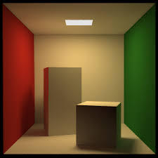
1 2 3 4 5 6 7 8 9 10 11 12 13 14 15 16 hittable_list cornell_box () {auto red = make_shared<lambertian>(make_shared<constant_texture>(vec3 (0.65 , 0.05 , 0.05 )));auto white = make_shared<lambertian>(make_shared<constant_texture>(vec3 (0.73 , 0.73 , 0.73 )));auto green = make_shared<lambertian>(make_shared<constant_texture>(vec3 (0.12 , 0.45 , 0.15 )));auto light = make_shared<diffuse_light>(make_shared<constant_texture>(vec3 (15 , 15 , 15 )));add (make_shared<yz_rect>(0 , 555 , 0 , 555 , 555 , green));add (make_shared<yz_rect>(0 , 555 , 0 , 555 , 0 , red));add (make_shared<xz_rect>(213 , 343 , 227 , 332 , 554 , light));add (make_shared<xz_rect>(0 , 555 , 0 , 555 , 0 , white));add (make_shared<xy_rect>(0 , 555 , 0 , 555 , 555 , white));add (make_shared<xz_rect>(0 , 555 , 0 , 555 , 555 , white));return objects;
下面是新的摄像机的参数:
mian.cc 1 2 3 4 5 6 7 8 9 10 const auto aspect_ratio = double vec3 lookfrom (278 , 278 , -800 ) ;vec3 lookat (278 ,278 ,0 ) ;vec3 vup (0 ,1 ,0 ) ;auto dist_to_focus = 10.0 ;auto aperture = 0.0 ;auto vfov = 40.0 ;camera cam (lookfrom, lookat, vup, vfov, aspect_ratio, aperture, dist_to_focus, 0.0 , 1.0 ) ;
我们会得到如下的结果:
这看上去都是噪点, 因为光太小了。我们还有一个问题: 一些墙壁的朝向反了。我们还没有让漫反射材质的正反两面有相同的表现。但cornell box的内外部是不同的模式。一个矩形物体的正面往往是$(1, 0, 0)$, $(0, 1, 0)$, 或者 $(0, 0, 1)$ 这几个方向。我们需要一种翻转矩形朝向的方法。所以让我们来一个新的hittable类吧, 别得啥都不干, 专门用来翻转正反面。
1 2 3 4 5 6 7 8 9 10 11 12 13 14 15 16 17 18 19 class flip_face :public hittable {public :flip_face (shared_ptr<hittable> p) : ptr (p) {}virtual bool hit (const ray& r, double t_min, double t_max, hit_record& rec) const if (!ptr->hit (r, t_min, t_max, rec))return false ;return true ;virtual bool bounding_box (double t0, double t1, aabb& output_box) const return ptr->bounding_box (t0, t1, output_box);public :
这是生成一个cornell box的代码:
diff 1 2 3 4 5 6 7 8 9 10 11 12 13 14 15 16 17 18 hittable_list cornell_box () {auto red = make_shared<lambertian>(make_shared<constant_texture>(vec3 (0.65 , 0.05 , 0.05 )));auto white = make_shared<lambertian>(make_shared<constant_texture>(vec3 (0.73 , 0.73 , 0.73 )));auto green = make_shared<lambertian>(make_shared<constant_texture>(vec3 (0.12 , 0.45 , 0.15 )));auto light = make_shared<diffuse_light>(make_shared<constant_texture>(vec3 (15 , 15 , 15 )));add (make_shared<flip_face>(make_shared<yz_rect>(0 , 555 , 0 , 555 , 555 , green)));add (make_shared<yz_rect>(0 , 555 , 0 , 555 , 0 , red));add (make_shared<xz_rect>(213 , 343 , 227 , 332 , 554 , light));add (make_shared<flip_face>(make_shared<xz_rect>(0 , 555 , 0 , 555 , 555 , white)));add (make_shared<xz_rect>(0 , 555 , 0 , 555 , 0 , white));add (make_shared<flip_face>(make_shared<xy_rect>(0 , 555 , 0 , 555 , 555 , white)));return objects;
看呀:
8. 实例 Cornell Box里面一般都有两个相对墙面有些角度的长方体。首先我们先把轴对齐的长方体图元做出来。每个长方体是由6个平面构成的:
box.h 1 2 3 4 5 6 7 8 9 10 11 12 13 14 15 16 17 18 19 20 21 22 23 24 25 26 27 28 29 30 31 32 33 34 35 36 37 38 class box :public hittable {public :box () {}box (const vec3& p0, const vec3& p1, shared_ptr<material> ptr);virtual bool hit (const ray& r, double t0, double t1, hit_record& rec) const virtual bool bounding_box (double t0, double t1, aabb& output_box) const aabb (box_min, box_max);return true ;public :box (const vec3& p0, const vec3& p1, shared_ptr<material> ptr) {add (make_shared<xy_rect>(p0.x (), p1.x (), p0.y (), p1.y (), p1.z (), ptr));add (make_shared<flip_face>(x (), p1.x (), p0.y (), p1.y (), p0.z (), ptr)));add (make_shared<xz_rect>(p0.x (), p1.x (), p0.z (), p1.z (), p1.y (), ptr));add (make_shared<flip_face>(x (), p1.x (), p0.z (), p1.z (), p0.y (), ptr)));add (make_shared<yz_rect>(p0.y (), p1.y (), p0.z (), p1.z (), p1.x (), ptr));add (make_shared<flip_face>(y (), p1.y (), p0.z (), p1.z (), p0.x (), ptr)));bool box::hit (const ray& r, double t0, double t1, hit_record& rec) const return sides.hit (r, t0, t1, rec);
现在我们可以加入两个长方体了(但是没有旋转的角度)
1 2 objects.add (make_shared<box>(vec3 (130 , 0 , 65 ), vec3 (295 , 165 , 230 ), white));add (make_shared<box>(vec3 (265 , 0 , 295 ), vec3 (430 , 330 , 460 ), white));
现在有:
现在我们有了这两个长方体, 为了让它看上去更加接近正宗 的Cornell Box, 我们还需要让他旋转一下。在光线追踪中, 我们时常使用实例(instance)来完成这个工作。实例是一种经过旋转过或者平移等操作的几何图元。在光线追踪中, 这其实很简单。我们并不需要去移动任何东西。相对的, 我们只需将射线。举例来说, 想象一个 平移 操作, 我们可以将位于原点的粉红色盒子所有的组成部分的的x值+2, 或者就把盒子放在那里, 然后在hit函数中, 相对的将射线的原点-2。(这也是我们在ray tracing中惯用的做法) 【译注: 射线原点-2计算出hit record后, 得到是左边盒子, 最后还要将计算结果+2, 才能获得正确的射入点(右边盒子)】
你把刚刚的这个操作当成是平移还是坐标系的转换都行, 随你的喜好。移动hittable类的translate的代码如下
1 2 3 4 5 6 7 8 9 10 11 12 13 14 15 16 17 18 19 20 21 22 23 24 25 26 27 28 29 30 31 32 33 34 class translate :public hittable {public :translate (shared_ptr<hittable> p, const vec3& displacement)ptr (p), offset (displacement) {}virtual bool hit (const ray& r, double t_min, double t_max, hit_record& rec) const virtual bool bounding_box (double t0, double t1, aabb& output_box) const public :bool translate::hit (const ray& r, double t_min, double t_max, hit_record& rec) const ray moved_r (r.origin() - offset, r.direction(), r.time()) ;if (!ptr->hit (moved_r, t_min, t_max, rec))return false ;set_face_normal (moved_r, rec.normal);return true ;bool translate::bounding_box (double t0, double t1, aabb& output_box) const if (!ptr->bounding_box (t0, t1, output_box))return false ;aabb (min () + offset,max () + offset);return true ;
旋转就没有那么容易理解或列出算式了。一个常用的图像技巧是将所有的旋转都当成是绕xyz轴旋转。首先, 让我们绕z轴旋转。这样只会改变xy而不会改变z值。
这里包含了一些三角几何. 我这里就不展开了。你要知道这其实很简单, 并不需要太多的几何知识, 你能在任何一本图形学的教材或者课堂笔记中找到它。绕z轴逆时针旋转的公式如下:
$$ x’ = \cos(\theta) \cdot x - \sin(\theta) \cdot y $$
这个公式的伟大之处在于它对任何$\theta$都成立, 你完全不用去考虑什么象限啊或者别的类似的东西。如果要顺时针旋转, 只需把$\theta$改成$-\theta$即可。来, 回想一下$\cos(\theta) = \cos(-\theta)$ 和 $\sin(-\theta) = -\sin(\theta)$, 所以逆运算的公式很简单。
类似的, 绕y轴旋转(也正是我们相对这两个长方体做的事情)的公式如下:
$$ x’ = \cos(\theta) \cdot x + \sin(\theta) \cdot z $$
绕x轴旋转的公式如下:
$$ y’ = \cos(\theta) \cdot y - \sin(\theta) \cdot z $$
和平移变换不同, 旋转时表面法向也发生了变化。所以在计算完hit函数后我们还要重新计算法向量。幸好对于旋转来说, 我们对法向量使用相同的公式变换一下即可。如果你加入了缩放(Scale), 那么这下事情就复杂多了。点击我们的网页 https://in1weekend.blogspot.com/ 了解详细信息。
对一个绕y轴的旋转变换来说, 我们有:
hittable.h 1 2 3 4 5 6 7 8 9 10 11 12 13 14 15 16 17 class rotate_y :public hittable {public :rotate_y (shared_ptr<hittable> p, double angle);virtual bool hit (const ray& r, double t_min, double t_max, hit_record& rec) const virtual bool bounding_box (double t0, double t1, aabb& output_box) const return hasbox;public :double sin_theta;double cos_theta;bool hasbox;
加上构造函数:
1 2 3 4 5 6 7 8 9 10 11 12 13 14 15 16 17 18 19 20 21 22 23 24 25 26 27 28 29 30 31 rotate_y::rotate_y (shared_ptr<hittable> *p, double angle) : ptr (p) {auto radians = degrees_to_radians (angle);sin (radians);cos (radians);bounding_box (0 , 1 , bbox);vec3 min ( infinity, infinity, infinity) ;vec3 max (-infinity, -infinity, -infinity) ;for (int i = 0 ; i < 2 ; i++) {for (int j = 0 ; j < 2 ; j++) {for (int k = 0 ; k < 2 ; k++) {auto x = i*bbox.max ().x () + (1 -i)*bbox.min ().x ();auto y = j*bbox.max ().y () + (1 -j)*bbox.min ().y ();auto z = k*bbox.max ().z () + (1 -k)*bbox.min ().z ();auto newx = cos_theta*x + sin_theta*z;auto newz = -sin_theta*x + cos_theta*z;vec3 tester (newx, y, newz) ;for (int c = 0 ; c < 3 ; c++) {ffmin (min[c], tester[c]);ffmax (max[c], tester[c]);aabb (min, max);
以及hit函数:
1 2 3 4 5 6 7 8 9 10 11 12 13 14 15 16 17 18 19 20 21 22 23 24 25 26 27 28 29 bool rotate_y::hit (const ray& r, double t_min, double t_max, hit_record& rec) const origin ();direction ();0 ] = cos_theta*r.origin ()[0 ] - sin_theta*r.origin ()[2 ];2 ] = sin_theta*r.origin ()[0 ] + cos_theta*r.origin ()[2 ];0 ] = cos_theta*r.direction ()[0 ] - sin_theta*r.direction ()[2 ];2 ] = sin_theta*r.direction ()[0 ] + cos_theta*r.direction ()[2 ];ray rotated_r (origin, direction, r.time()) ;if (!ptr->hit (rotated_r, t_min, t_max, rec))return false ;0 ] = cos_theta*rec.p[0 ] + sin_theta*rec.p[2 ];2 ] = -sin_theta*rec.p[0 ] + cos_theta*rec.p[2 ];0 ] = cos_theta*rec.normal[0 ] + sin_theta*rec.normal[2 ];2 ] = -sin_theta*rec.normal[0 ] + cos_theta*rec.normal[2 ];set_face_normal (rotated_r, normal);return true ;
并且修改一下生成cornell box的Cornell函数:
1 2 3 4 5 6 7 8 9 shared_ptr<hittable> box1 = make_shared<box>(vec3 (0 , 0 , 0 ), vec3 (165 , 330 , 165 ), white);15 );vec3 (265 ,0 ,295 ));add (box1);vec3 (0 ,0 ,0 ), vec3 (165 ,165 ,165 ), white);-18 );vec3 (130 ,0 ,65 ));add (box2);
最后得到:
9. 体积体 给光线追踪器加入烟/雾/水汽是一件很不错的事情。这些东西常常被称为体积体(volumes)或者可参与介质(participating media)。次表面散射(sub surface scatter, SSS)是另一个不错的特性, 有点像物体内部的浓雾。加入这部分内容会导致代码结构的混乱。因为体积体和平面表面是完全不同的两种东西。但我们有一个可爱的小技巧: 将体积体表示为一个随机表面。一团烟雾在其实可以用一个概率上不确定在什么位置的平面来代替。当你看到代码后, 你就会更有感觉了。
首先让我们来生成一个固定密度的体积体。光线可以在体积体内部发生散射, 也可以像图中的中间那条射线一样直接穿过去。体积体越薄越透明, 直接穿过去的情况就越有可能会发生。光线在体积体中直线传播所经过的距离也决定了光线采用图中哪种方式通过体积体。
当光线射入体积体时, 它可能在任意一点发生散射。体积体越浓, 越可能发生散射。在任意微小的距离差$\Delta L$发生散射的概率如下:
$$ \text{probability} = C \cdot \Delta L $$
其中$C$是体积体的光学密度比例常数。 经过了一系列不同的等式运算, 你将会随机的得到一个光线发生散射的距离值。如果根据这个距离来说, 散射点在体积体外, 那么我们认为没有相交, 不调用hit函数。对于一个静态的体积体来说, 我们只需要他的密度C和边界。我会用另一个hittable物体来表示体积体的边界:
1 2 3 4 5 6 7 8 9 10 11 12 13 14 15 16 17 18 19 class constant_medium :public hittable {public :constant_medium (shared_ptr<hittable> b, double d, shared_ptr<texture> a)boundary (b), neg_inv_density (-1 /d)virtual bool hit (const ray& r, double t_min, double t_max, hit_record& rec) const virtual bool bounding_box (double t0, double t1, aabb& output_box) const return boundary->bounding_box (t0, t1, output_box);public :double neg_inv_density;
对于散射的方向来说, 我们采用各项同性(isotropic)的随机单位向量大法
1 2 3 4 5 6 7 8 9 10 11 12 13 14 15 class isotropic :public material {public :isotropic (shared_ptr<texture> a) : albedo (a) {}virtual bool scatter ( const ray& r_in, const hit_record& rec, vec3& attenuation, ray& scattered ) const ray (rec.p, random_in_unit_sphere (), r_in.time ());value (rec.u, rec.v, rec.p);return true ;public :
hit函数如下:
1 2 3 4 5 6 7 8 9 10 11 12 13 14 15 16 17 18 19 20 21 22 23 24 25 26 27 28 29 30 31 32 33 34 35 36 37 38 39 40 41 42 43 44 45 46 bool constant_medium::hit (const ray& r, double t_min, double t_max, hit_record& rec) const const bool enableDebug = false ;const bool debugging = enableDebug && random_double () < 0.00001 ;if (!boundary->hit (r, -infinity, infinity, rec1))return false ;if (!boundary->hit (r, rec1.t+0.0001 , infinity, rec2))return false ;if (debugging) std::cerr << "\nt0=" << rec1.t << ", t1=" << rec2.t << '\n' ;if (rec1.t < t_min) rec1.t = t_min;if (rec2.t > t_max) rec2.t = t_max;if (rec1.t >= rec2.t)return false ;if (rec1.t < 0 )0 ;const auto ray_length = r.direction ().length ();const auto distance_inside_boundary = (rec2.t - rec1.t) * ray_length;const auto hit_distance = neg_inv_density * log (random_double ());if (hit_distance > distance_inside_boundary)return false ;at (rec.t);if (debugging) {"hit_distance = " << hit_distance << '\n' "rec.t = " << rec.t << '\n' "rec.p = " << rec.p << '\n' ;vec3 (1 ,0 ,0 ); true ; return true ;
我们一定要小心与边界相关的逻辑, 因为我们要确保当射线原点在体积体内部时, 光线依然会发生散射。在云中, 光线反复发生散射, 这是一种很常见的现象。
另外, 上述代码只能确保射线只会射入体积体一次, 之后再也不进入体积体的情况。换句话说, 它假定体积体的边界是一个凸几何体。所以这个狭义的实现只对球体或者长方体这样的物体生效。但是对于当中有洞的那种形状, 如甜甜圈就不行了。写一个能处理任意形状的实现是完全可行的, 但我们把这部分内容留给我们的读者作为练习。
如果我们将两个长方体替换为烟和雾(深色与浅色的粒子)并使用一个更大的灯光(同时更加昏暗以至于不会炸了这个场景)让场景更快的融合在一起。
1 2 3 4 5 6 7 8 9 10 11 12 13 14 15 16 17 18 19 20 21 22 23 24 25 26 27 28 29 30 hittable_list cornell_smoke () {auto red = make_shared<lambertian>(make_shared<constant_texture>(vec3 (0.65 , 0.05 , 0.05 )));auto white = make_shared<lambertian>(make_shared<constant_texture>(vec3 (0.73 , 0.73 , 0.73 )));auto green = make_shared<lambertian>(make_shared<constant_texture>(vec3 (0.12 , 0.45 , 0.15 )));auto light = make_shared<diffuse_light>(make_shared<constant_texture>(vec3 (7 , 7 , 7 )));add (make_shared<flip_face>(make_shared<yz_rect>(0 , 555 , 0 , 555 , 555 , green)));add (make_shared<yz_rect>(0 , 555 , 0 , 555 , 0 , red));add (make_shared<xz_rect>(113 , 443 , 127 , 432 , 554 , light));add (make_shared<flip_face>(make_shared<xz_rect>(0 , 555 , 0 , 555 , 555 , white)));add (make_shared<xz_rect>(0 , 555 , 0 , 555 , 0 , white));add (make_shared<flip_face>(make_shared<xy_rect>(0 , 555 , 0 , 555 , 555 , white)));vec3 (0 ,0 ,0 ), vec3 (165 ,330 ,165 ), white);15 );vec3 (265 ,0 ,295 ));vec3 (0 ,0 ,0 ), vec3 (165 ,165 ,165 ), white);-18 );vec3 (130 ,0 ,65 ));add (0.01 , make_shared<constant_texture>(vec3 (0 ,0 ,0 ))));add (0.01 , make_shared<constant_texture>(vec3 (1 ,1 ,1 ))));return objects;
我们会得到:
10. 一个测试所有新特性的场景 让我们把所有东西放在一起吧!使用一个薄雾盖住所有东西, 并加入一个蓝色的次表面反射球体(这种说法不太清楚, 实际上次表面材质就是在电介质内部填充体积体)。现在这个渲染器的最大局限就是没有阴影光线。但是因此我们能不花代价的得到散焦和次表面。这是一把设计上的双刃剑。
main.cc 1 2 3 4 5 6 7 8 9 10 11 12 13 14 15 16 17 18 19 20 21 22 23 24 25 26 27 28 29 30 31 32 33 34 35 36 37 38 39 40 41 42 43 44 45 46 47 48 49 50 51 52 53 54 55 56 57 58 59 60 61 62 63 64 65 66 67 68 69 70 hittable_list final_scene () {auto ground =vec3 (0.48 , 0.83 , 0.53 )));const int boxes_per_side = 20 ;for (int i = 0 ; i < boxes_per_side; i++) {for (int j = 0 ; j < boxes_per_side; j++) {auto w = 100.0 ;auto x0 = -1000.0 + i*w;auto z0 = -1000.0 + j*w;auto y0 = 0.0 ;auto x1 = x0 + w;auto y1 = random_double (1 ,101 );auto z1 = z0 + w;add (make_shared<box>(vec3 (x0,y0,z0), vec3 (x1,y1,z1), ground));add (make_shared<bvh_node>(boxes1, 0 , 1 ));auto light = make_shared<diffuse_light>(make_shared<constant_texture>(vec3 (7 , 7 , 7 )));add (make_shared<xz_rect>(123 , 423 , 147 , 412 , 554 , light));auto center1 = vec3 (400 , 400 , 200 );auto center2 = center1 + vec3 (30 ,0 ,0 );auto moving_sphere_material =vec3 (0.7 , 0.3 , 0.1 )));add (make_shared<moving_sphere>(center1, center2, 0 , 1 , 50 , moving_sphere_material));add (make_shared<sphere>(vec3 (260 , 150 , 45 ), 50 , make_shared<dielectric>(1.5 )));add (make_shared<sphere>(vec3 (0 , 150 , 145 ), 50 , make_shared<metal>(vec3 (0.8 , 0.8 , 0.9 ), 10.0 )auto boundary = make_shared<sphere>(vec3 (360 , 150 , 145 ), 70 , make_shared<dielectric>(1.5 ));add (boundary);add (make_shared<constant_medium>(0.2 , make_shared<constant_texture>(vec3 (0.2 , 0.4 , 0.9 ))vec3 (0 , 0 , 0 ), 5000 , make_shared<dielectric>(1.5 ));add (make_shared<constant_medium>(.0001 , make_shared<constant_texture>(vec3 (1 ,1 ,1 ))));int nx, ny, nn;auto tex_data = stbi_load ("earthmap.jpg" , &nx, &ny, &nn, 0 );auto emat = make_shared<lambertian>(make_shared<image_texture>(tex_data, nx, ny));add (make_shared<sphere>(vec3 (400 ,200 , 400 ), 100 , emat));auto pertext = make_shared<noise_texture>(0.1 );add (make_shared<sphere>(vec3 (220 ,280 , 300 ), 80 , make_shared<lambertian>(pertext)));auto white = make_shared<lambertian>(make_shared<constant_texture>(vec3 (0.73 , 0.73 , 0.73 )));int ns = 1000 ;for (int j = 0 ; j < ns; j++) {add (make_shared<sphere>(vec3::random (0 ,165 ), 10 , white));add (make_shared<translate>(0.0 , 1.0 ), 15 ),vec3 (-100 ,270 ,395 )return objects;
每个像素点采样10,000次, 得到下图的结果:
现在你可以合上这本书, 开始生成属于你自己的炫酷图片! 在 https://in1weekend.blogspot.com/ 获取后续阅读内容和新特性, 如果你在阅读过程中遇到了问题, 或对本书有什么看法或评价, 或者想分享你的炫酷图片, 欢迎发送邮件到 ptrshrl@gmail.com